Linear Regression XL: All Possible Subsets
Start
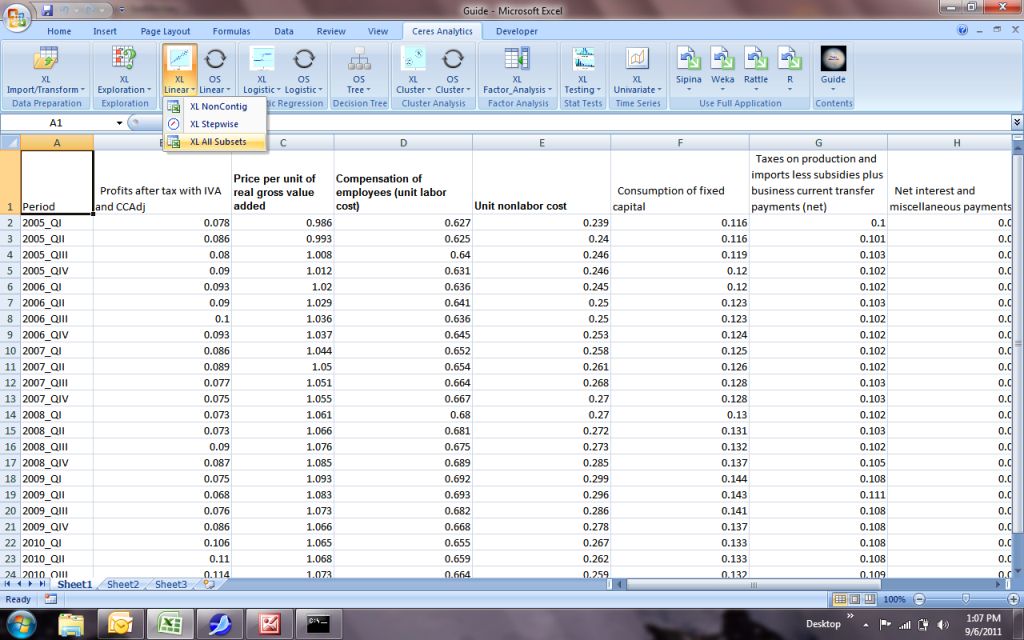
In the "Linear Regression" group, "XL Linear" tab, choose "XL All Subsets" from the menu.
1.
You'll be prompted for "Y" (in an X-Y context, the dependent variable). Begin by clicking on its title...
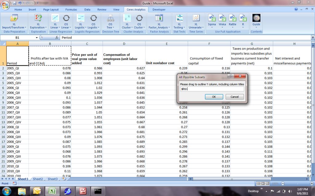
1a.
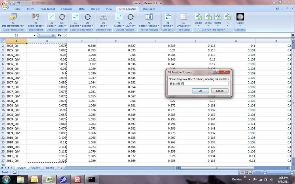
...then drag through the column. The easy shortcut to the bottom of the column is <CONTROL><SHIFT><DOWN>. When you've identified the range, you'll see the range endpointsidentified in the pop-up box:
2.
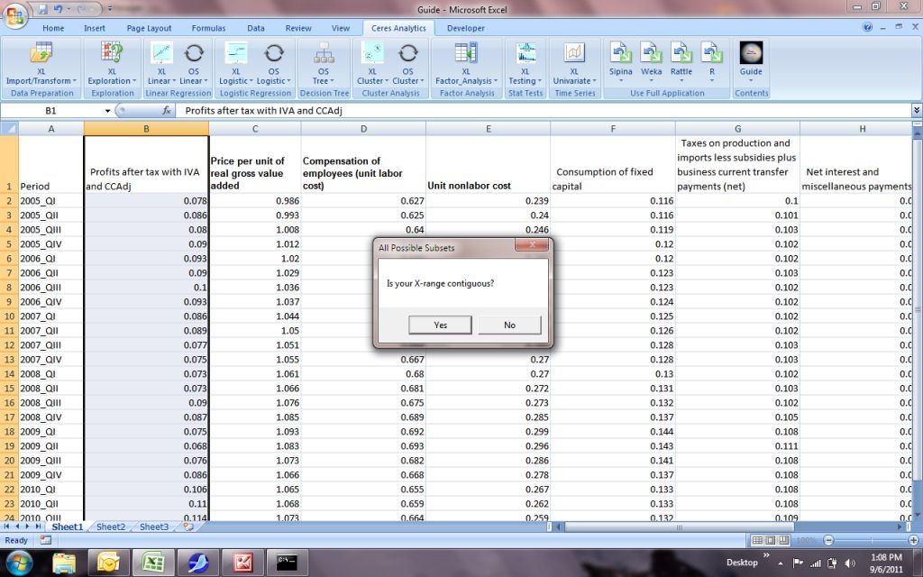
The next question is whether the X-range is contiguous. That is, whether all of the independent variables are side-by-side, on the same sheet.
You can answer "No" to choose columns from different places on a worksheet, and from different worksheets.
In this example, they are all together, so we'll choose "Yes".
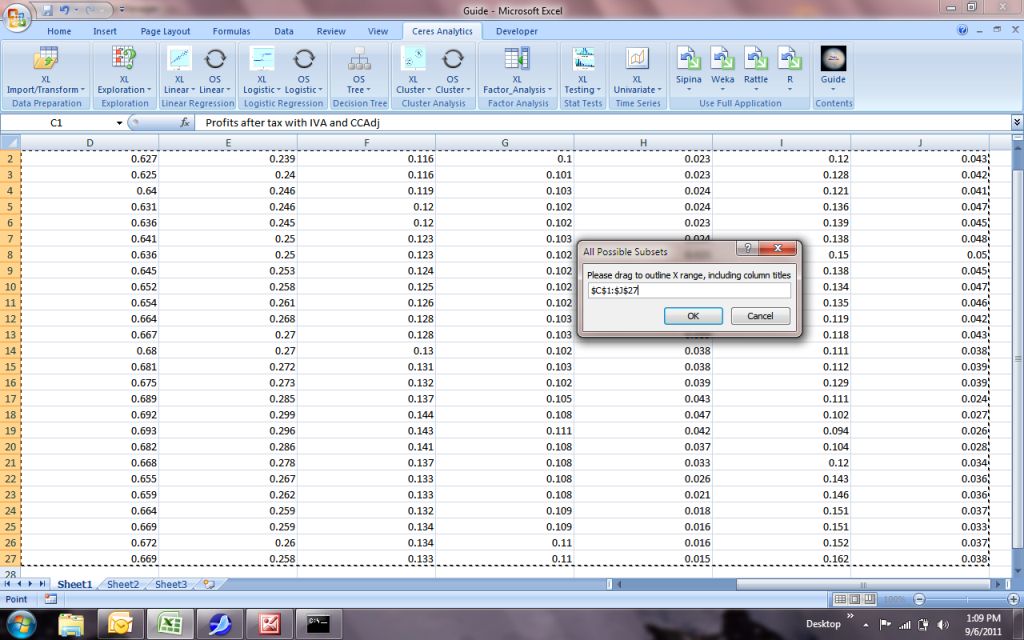
3.
Next you'll be prompted to drag through the X range.
The process is the same as for the Y range, except that you can use <CONTROL><SHIFT><RIGHT> to go to the end of data that extend rightward.
4.
Next, you'll be asked for the minimum number of predictors (X variables) to include in each equation.
Regression equations for all possible subsets with this minimum number of predictors will be tested.
In this example, we'll answer 1:

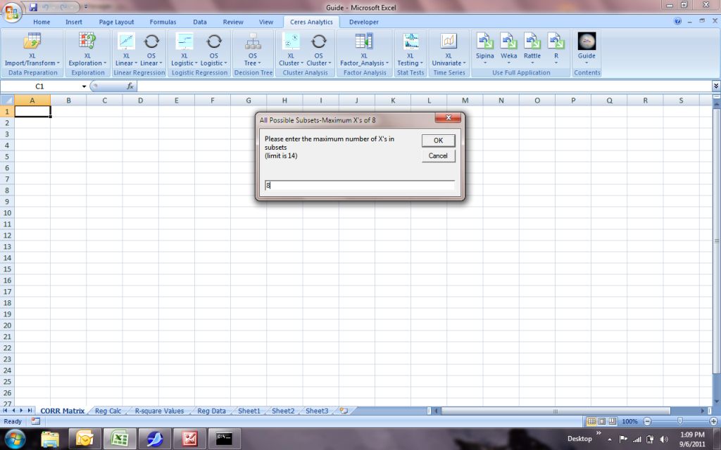
5.
Just like the minimum, you'll be asked for the maximum number of predictors. Note that the number of predictors available is in the title bar of the pop-up.
The lower the maximum, the fewer models will be fit. As the maximum increases, the number of models increases exponentially.
In this example, we'll choose 8 (the maximum number of predictors available).
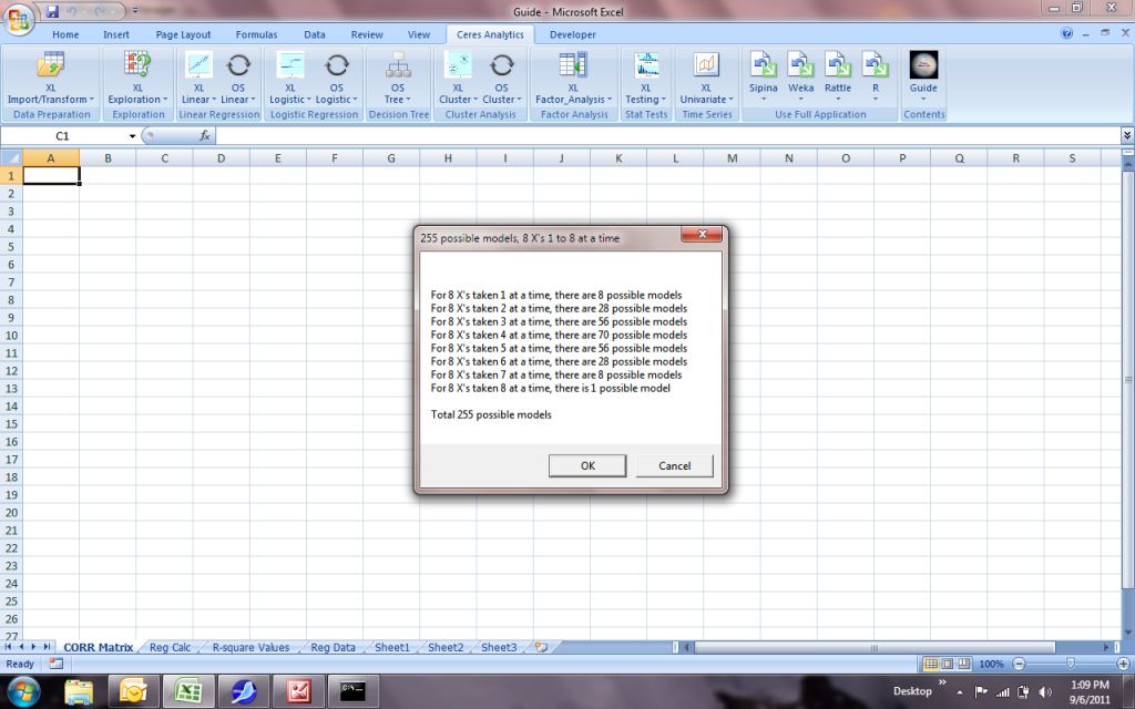
6.
To avoid excessively long computation times, you'll be given an option to stop the run.
This option shows how the number of regression equations was calculated.
If you stop the run, you might wish to re-run with a lower maximum number of predictors. The number of regression equations will be reduced by the number associated with each of the higher maxima that you omit.
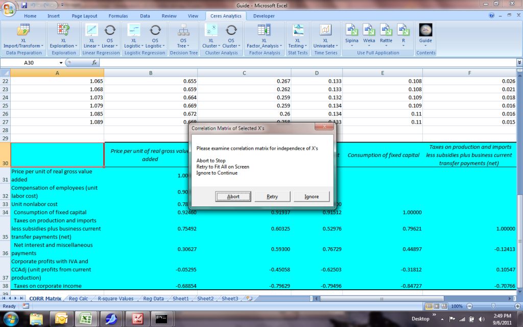
7.
The correlation matrix of the predictors is shown. You can resize the matrix for closer inspection, if wanted.
8.
The resulting equations will be presented from the minimum number of predictors (here, 1) to the maximum number of predictors (here, 8).
Within each quantity of predictors, the equations will be sorted by descending R-square. The predictors in the model are listed in Column C ("In Model").
The equations with Adjusted R-squares greater than or equal to 0.70 will be color-coded as folllows:
| Adjusted R-Square Value |
Color |
| >=.90 |
Aqua Blue |
| >=.80 |
Yellow |
| >=.70 |
Lime Green |
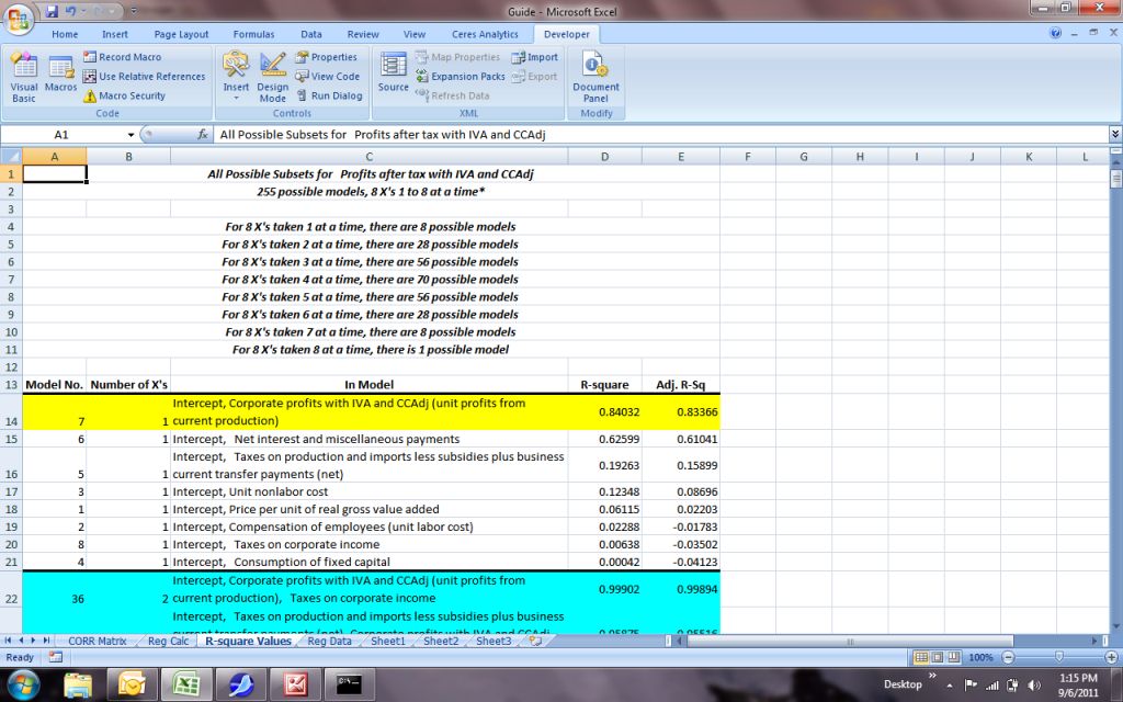
9.
Scrolling down we can see more of the results:
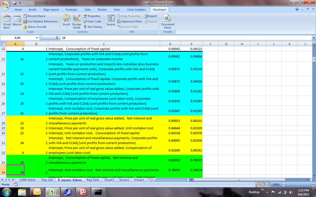
10.
And at the bottom, the equation with the maximum number of predictors, along with the list of predictors we identified when we started:
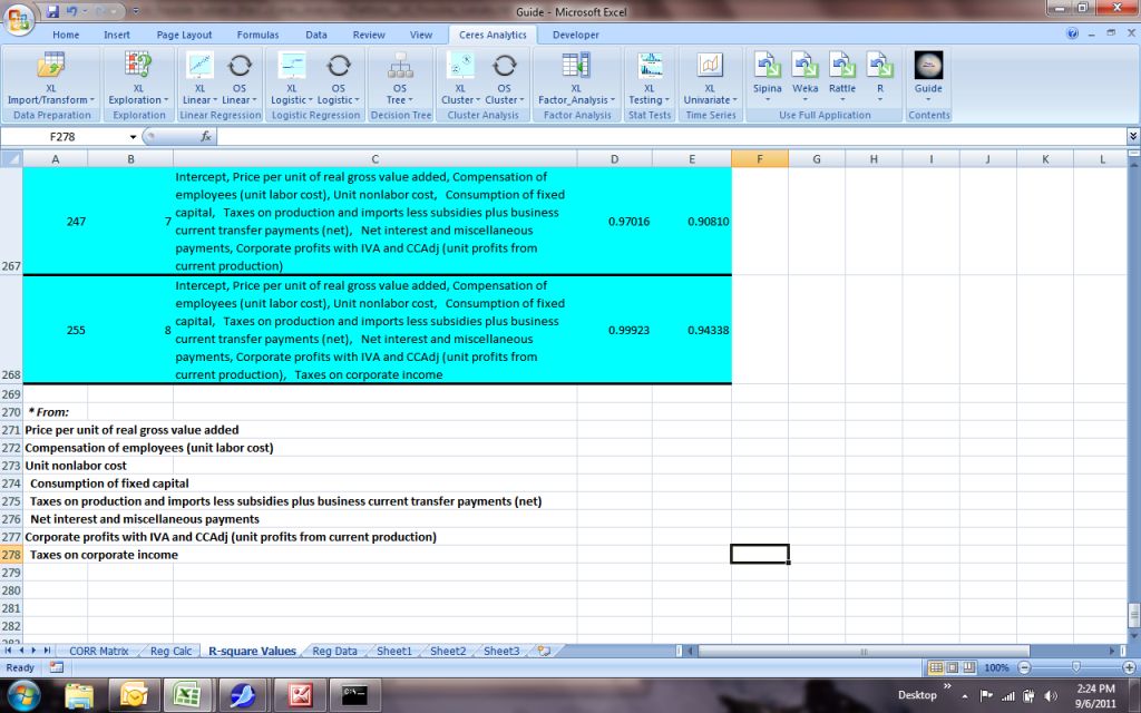
Conclusion
The All Possible Subsets algorithm gives insight into the impacts of different combinations of predictors.
Given these insights, the analyst can follow up the most promising equations with detailed, individual runs to examine statistical significance and signs of coefficients.