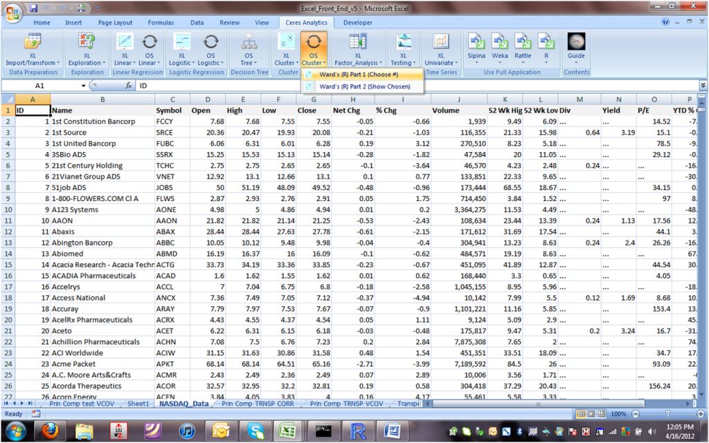
Cluster Analysis OS: Part 1 (Exploratory)
2.
If you've been working in the Ceres Platform, you'll be asked whether to continue with the same folder....
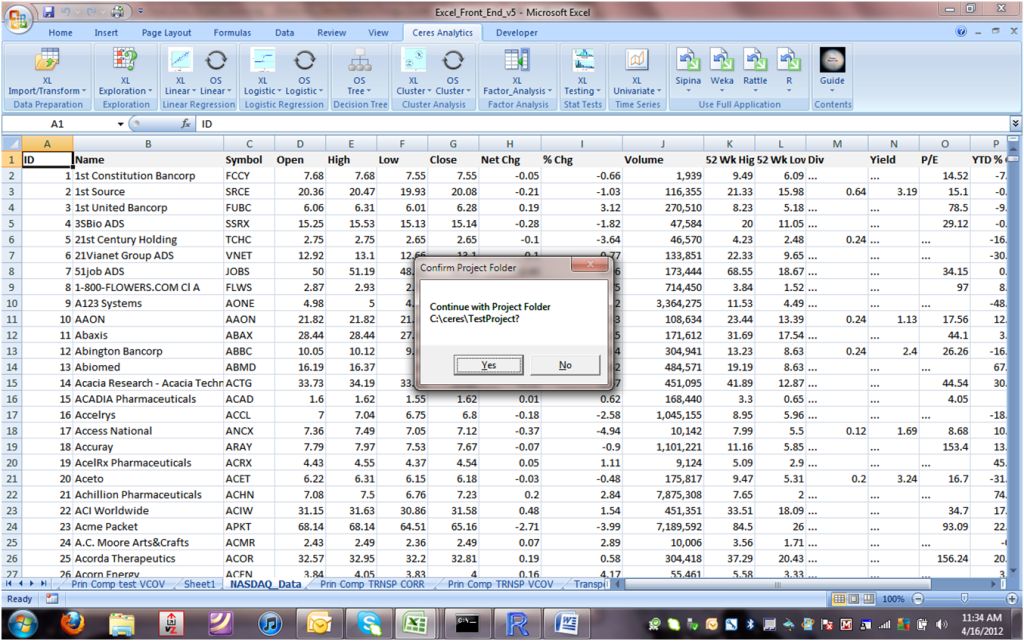
3.
Whether or not you've been working in the Ceres platform, you'll see the control panel to verify, or to initiate, your project folders:
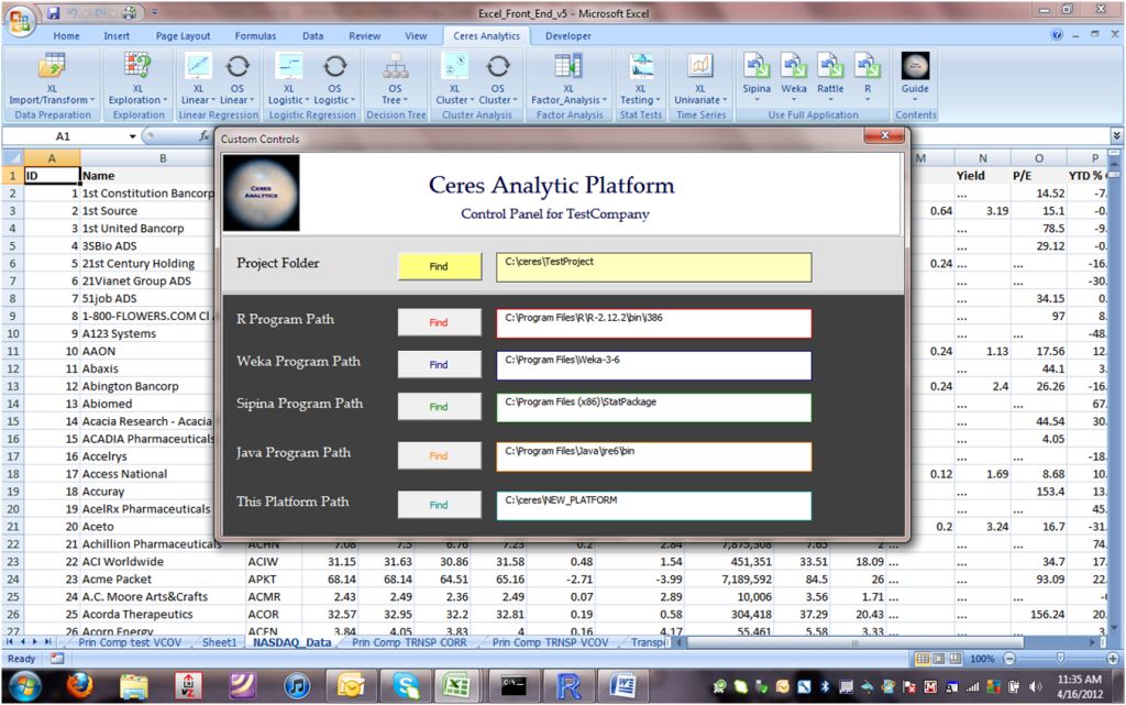
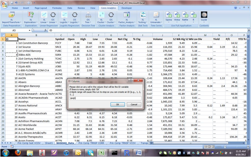
4.
You'll be asked to provide an ID column. Here, there's one in the data. If you don't have one, there's an option for automatic creation of an ID.
Note: In this example, the Ceres Platform is configured to work with input data from an Excel workbook.
In larger-scale applications, the Platform can be directed to other sources, such as a relational database management system.
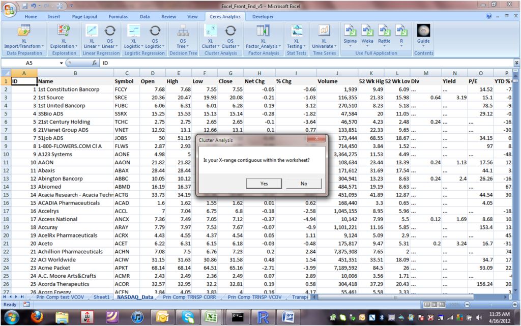
5.
Next you'll be asked if the data are contiguous. If they're not, you'll get to select different columns (or column blocks) to assemble a custom set of variables.
The Ceres Platform prompts you for a range of "X" data, reflecting that the data that determine the clusters are independent variables.
The cluster designation, in contrast, is dependent on the "X"s.
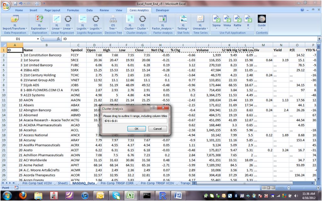
6.
Next you'll be prompted to drag through the data range.
You can use <CONTROL><SHIFT><DOWN> to go to the end of data.
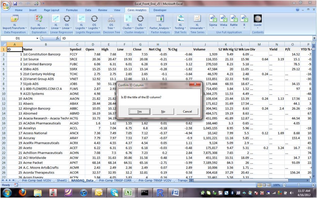
7.
There's a double-check on the ID column. The ID will be used to attach the cluster identifier to each observation.
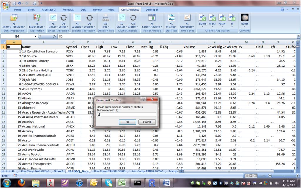
8.
The Ceres algorithm will evaluate alternative solutions, each with a different number of clusters. You'll be asked first for the minimum number of clusters:
9.
Then you'll be asked for the maximum number of clusters:
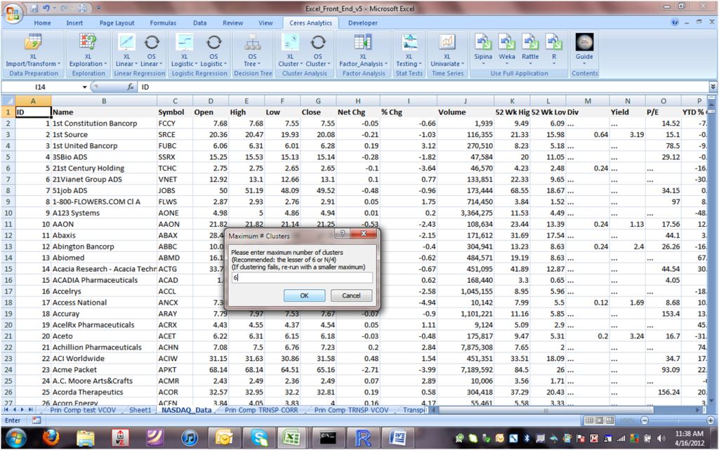
10.
The Ceres Platform will modify the base R script that Ceres developed. The script includes clustering features from a number of different R packages.
The methods and algorithms reflect Ceres' research and experience. For example:
- Ward's method is used because it tends toward groups of equal size.
- We rarely obtain equally sized groups
- Rather, the contrasts between the groups are definitive
- A few key statistical measures help to define the
"best" number of clusters. Notably:
- When the Within:Between Ratio "flatlines" after
steep drop(s), additional clusters are often not
useful
- A minimum silhouette score is optimal, but when the values are close, there is room to rely on other measures
- The height of the branches in the dendogram (tree picture) show how well-defined the clusters are:
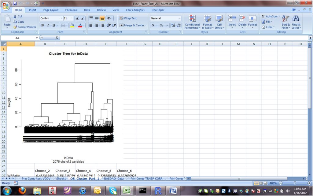
11.
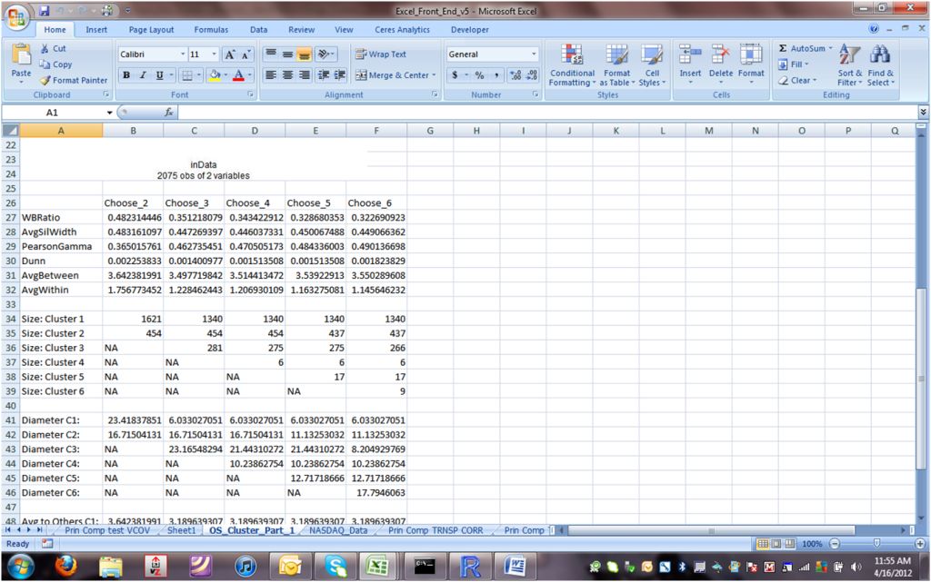
Scrolling down, we can see the measures noted above:
- The Within:Between Ratio ("WBRatio" at row 27) flatlines after 3 clusters, suggesting that 4 is too many.
- The Average Silhoutte Width ("AvgSilWidth") at row 28 is virtually constant from 3 to 6 clusters
Those few observations would otherwise be contained in the smaller two of the three clusters.
Conclusion
With exploratory analysis suggesting a three-cluster solution, we can now examine cluster profiles, cohesion and dispersion in Part 2.